NHL Data
I’ve only fairly recently come to like ice hockey over the last 4 years. We have a really good team in the area I live, so that makes it easier to watch. I also like the style of hockey that team plays; whicht tends to favor speed and skill over heavy defense and slamming the other team into the walls (although they also spend too much passing and not putting the puck on the net). I think I like ice hockey for a couple of reasons. The game is constantly in action. While I like watching American Football, the game lasts four hours with too many commercial breaks. I think someone calculated that there is only 30 minutes of actual playing time in a game. Ice hockey also has an international flavor to it given the NHL includes two countries. Players also come from many different countries (Sweden, Switzerland, Canada, Russia just to name a few). It’s also the only sport I’ve seen make a comment on climate change through a commercial. I only saw it once, but it made it’s point through the problem of frozen ponds disapearing as the earth gets warmer. Of course, having ice rinks in Florida, Arizona, and Las Vegas might seem a little hypocritical.
It is fair to say that ice hockey is a low scoring game. For example, a local promotion advertises if the local NHL team scores 5 goals in a game then you will get a discount on your tires. This, of course, happens rarely. A number of factors contribute to the low score: the quality of the goalie, the size of the net, the skill of the skaters on the respective teams, and the size of the goalie’s equipment. They recently changed the rules to make the leg padding smaller in hopes it would increase the number of goals in the game. I’m not sure why there is a push to score more goals. Maybe it is to try and increase the market share, with the idea that American Football scores a lot of points.
However, what I’m intersted in is the effect of that first goal. It, intuitively, would seem that it makes it very important. You’ve gone from being difficult to win at even 0-0 to very difficult to win. One thing that might mediate this, is if you get that equalizer, and tie the game. Potentially pushing to overtime. Of course, a second goal then makes it even more difficult for the other team to win.
When I initially looked at the problem, I found very little research into the effect of the first goal in ice hockey. I admit this was a few years ago, and there may have been some studies since then. At the same time, it is such an intuitive thing, it may just be overlooked. On the other hand, there seems to be less analytic focus on ice hockey. Probably because the NHL is the fifth most popular sport in the US (https://en.wikipedia.org/wiki/Sports_in_the_United_States#Popular_team_sports). American Football, Basketball, Baseball, and Soccer all come first in popularity. Baseball has a long history of sabermetrics, and basketball has developed SportVue (I think they are starting to use it in the NHL too). You don’t hear about American Football analytics that much, or at least I haven’t.
So with all that in mind, I decided to do a mini analysis of the importance of scoring first in the NHL. I also wanted to look at some side questions such as who are the players that might be best at scoring first, and what are the effects of home ice advantage. To begin, I will just download and summarize the data.
Note:
This is all meant for fun. I’ve never played ice hockey, and am a casual watcher. I am not recommending using this information for player evaluation, but will talk about how this may be useful for developing strategy.
from nhlscrapi.games.game import GameKey, Game
from nhlscrapi.games.cumstats import Score
from nhlscrapi.games.playbyplay import PlayByPlay
from nhlscrapi.games.events import EventType
import cPickle as pickle
import pandas as pd
import numpy as np
from statsmodels.graphics.mosaicplot import mosaic
import seaborn as sns
import matplotlib.pyplot as plt
import re
from scipy.stats import poisson
%matplotlib inline
sns.set()
When I looked at this a few years ago, I initially used the R library for a first crack at this, but have switched to the python version. I admit I didn’t find it that user friendly. There were classes for everything and not very clear documentation. For example, trying to get every game for a season required an index for the game, but I couldn’t find a function to get me a list. The library doesn’t throw an error when you use a game index that doesn’t exist. Hence, it takes creating a GameKey object, a Game object, and then seeing if the matchup dictionary exists to see if the class actually loaded.
#depending on the season there were some odd problems with the the team names
def checkTeam(name):
    if name == "VEGAS GOLDEN KNIGHTS":
        name = "VGK"
    if name == "PHO" or "ARI":
        name = "PHX"
    name = name.replace(".","")
    name = name.strip()
    return name
The following code gets all the regular season games from 2014 to 2018. I skipped the 2013 season because it was shortened.
It creates a list of each game organized by home and away teams. It grams the team, who one, who scored first and second, whether it was a home game, overtime, total number of goals, and the penalty count.
It also grabs the full description for the play event of the first goal. I’ll use that to pull out the players that score the first goal.
games = []

index = 1
for yr in range(2014,2019):
    print yr
    index = 1

    games = []
    firstGoalDesc = []
    while 1:
        #print index
        gk = GameKey(yr,2,index)
        gkstr = '%s%s%s'%(yr,2,index)
        gda = {'gamekey':gkstr,'team':'','won':-1,'scoredfirst':-1,'scoredsecond':-1,'home':0,
               'overtime':-1,'goals':-1,'period':-1,'overtime':0,'penaltycount':0}
        gdh = {'gamekey':gkstr,'team':'','won':-1,'scoredfirst':-1,'scoredsecond':-1,'home':1,
               'overtime':-1,'goals':-1,'period':-1,'overtime':0,'penaltycount':0}
        g = Game(gk)
        g.load_all()
        if g.matchup:
            try:

                gdh['team'] = checkTeam(g.matchup['home'])
                gda['team']=  checkTeam(g.matchup['away'])
                gda['goals'] = int(g.matchup['final']['away'])
                gdh['goals'] = int(g.matchup['final']['home'])
                if gda['goals']>gdh['goals']:
                    gdh['won'] = 0
                    gda['won'] = 1
                else:
                    gdh['won'] = 1
                    gda['won'] = 0
                firstGoal = 0
                for p in g.plays:
                    if p.event.event_type == EventType.Penalty:
                        team = checkTeam(p.event.desc[:3])
                        if team == gda['team']:
                            gda['penaltycount'] += 1
                        elif team == gdh['team']:
                            gdh['penaltycount'] += 1
                    if p.event.event_type == EventType.Goal:
                        if firstGoal == 0:
                            #print p.event.event_type
                            #print p.period
                            #print p.event.desc
                            gda['period'] = p.period
                            gdh['period'] = p.period
                            firstGoalDesc.append((yr,p.period,p.event.desc))
                            team = checkTeam(p.event.desc[:3])

                            if team == gda['team']:
                                gda['scoredfirst'] = 1
                                gdh['scoredfirst'] = 0
                            elif team == gdh['team']:
                                gdh['scoredfirst'] = 1
                                gda['scoredfirst'] = 0
                            firstGoal =1
                        elif firstGoal ==1:
                            team = checkTeam(p.event.desc[:3])
                            if team == gda['team']:
                                gda['scoredsecond'] = 1
                                gdh['scoredsecond'] = 0
                            elif team == gdh['team']:
                                gdh['scoredsecond'] = 1
                                gda['scoredsecond'] = 0
                            firstGoal = 2
                        if p.period > 3:
                            gda['overtime'] = 1
                            gdh['overtime'] = 1
                games.append(gdh)
                games.append(gda)
            except:
                print g.matchup
            index+=1
            del g
            del gk

        else:
            print "None %s"%gkstr
            break
        #print index
        #if index > 5:
                #break
        if index % 20 == 0:
            print index
    #if yr == 2014:
        #break
    pickle.dump(games,open("allGames%s.p"%yr,'wb'))
    pickle.dump(firstGoalDesc,open("firstGoalDesc%s.p"%yr,'wb'))
Of course I ran into some problems when I started to review the game. These seem to revolve around games that had overtimes or the wrong team name. So this cleaned up some of the errors. For efficiency you could combine these when you scrape them.
for yr in range(2014,2019):
    gs = pickle.load(open("allGames%s.p"%yr,'rb'))
    for i in range(0,len(gs),2):
        team1 = gs[i]
        team2 = gs[i+1]
        gkstr = team1['gamekey']
        if team1['team'] == "PHO":
            team1['team'] = checkTeam(team1['team'])
            print checkTeam(team1['team'])
        if team2['team'] == "PHO":
            team2['team'] = checkTeam(team2['team'])
            print checkTeam(team1['team'])

        if team1['scoredfirst']==-1 or team2['scoredfirst']==-1:
            #print team1
            #print team2
            print (gkstr[:4],gkstr[4:5],gkstr[5:])
            gk = GameKey(int(gkstr[:4]),int(gkstr[4:5]),int(gkstr[5:]))
            g = Game(gk)
            g.load_all()
            if g.matchup:
                firstGoal = 0
                for p in g.plays:
                    if p.event.event_type == EventType.Goal:
                        if firstGoal == 0:
                            team = checkTeam(p.event.desc[:3])
                            if team==team1['team']:
                                team1['scoredfirst'] = 1
                                team2['scoredfirst'] = 0
                            elif team == team2['team']:
                                team2['scoredfirst'] = 1
                                team1['scoredfirst'] = 0
                            firstGoal =1
                        elif firstGoal ==1:
                            team = checkTeam(p.event.desc[:3])
                            if team == team1['team']:
                                team1['scoredsecond'] = 1
                                team2['scoredsecond'] = 0
                            elif team == team2['team']:
                                team2['scoredsecond'] = 1
                                team1['scoredsecond'] = 0
                            firstGoal = 2
                if firstGoal == 0:
                    print "%s no goals scored?"%gkstr
                    print g.matchup
                    if max(team1['goals'],team2['goals']) ==1:
                        if team1['won'] == 1:
                            team1['scoredfirst'] = 1
                            team1['scoredsecond']=0
                            team2['scoredfirst'] = 0
                            team2['scoredsecond']=0
                            team2['period']=4
                            team1['period']=4
                        elif team2['won'] == 1:
                            team2['scoredfirst'] = 1
                            team2['scoredsecond']=0
                            team1['scoredfirst'] = 0
                            team1['scoredsecond']=0
                            team2['period']=4
                            team1['period']=4
                if firstGoal == 1:
                    print "%s no second goal"%gkstr
                    if max(team1['goals'],team2['goals'])<2:
                        team2['scoredsecond'] = 0
                        team1['scoredsecond'] = 0
        if team1['scoredsecond']==-1 or team2['scoredsecond']==-1:
            if max(team1['goals'],team2['goals'])==1:
                team2['scoredsecond'] = 0
                team1['scoredsecond'] = 0
            else:
                print (gkstr[:4],gkstr[4:5],gkstr[5:])
                gk = GameKey(int(gkstr[:4]),int(gkstr[4:5]),int(gkstr[5:]))
                g = Game(gk)
                g.load_all()
                if g.matchup:
                    firstGoal = 0
                    period = 0
                    for p in g.plays:
                        period = p.period
                        if p.event.event_type == EventType.Goal:
                            if firstGoal == 0:
                                firstGoal =1
                            elif firstGoal ==1:
                                team = checkTeam(p.event.desc[:3])
                                if team == team1['team']:
                                    team1['scoredsecond'] = 1
                                    team2['scoredsecond'] = 0
                                elif team == team2['team']:
                                    team2['scoredsecond'] = 1
                                    team1['scoredsecond'] = 0
                                firstGoal = 2
                    if firstGoal == 1:
                        if max(team1['goals'],team2['goals'])<2:
                            team2['scoredsecond'] = 0
                            team1['scoredsecond'] = 0

                        if team1['overtime'] == 1:
                            if team1['won'] == 1:
                                team2['scoredsecond'] = 0
                                team1['scoredsecond'] = 1
                            else:
                                team2['scoredsecond'] = 1
                                team1['scoredsecond'] = 0
            gs[i] = team1
            gs[i+1] = team2

    pickle.dump(gs,open("allGamesF%s.p"%yr,'wb'))
You could look at these individually as seasons, or pool them for multiple seasons.
allCombine = []
for yr in range(2014,2019):
    gs = pickle.load(open("allGamesF%s.p"%yr,'rb'))
    allCombine+= gs
len(allCombine)
12356
This loads the list into a dataframe, and checks for some missing values. These should be all zero at this point.
df = pd.DataFrame(allCombine)
df.head()
print df[(df['scoredfirst']==-1)].count()
print df[(df['period']==-1)].count()
print df[(df['scoredsecond']==-1)].count()
print df.describe()
print df[(df['scoredfirst']==1) &(df['won']==1)].count()
gamekey         0
goals           0
home            0
overtime        0
penaltycount    0
period          0
scoredfirst     0
scoredsecond    0
team            0
won             0
dtype: int64
gamekey         0
goals           0
home            0
overtime        0
penaltycount    0
period          0
scoredfirst     0
scoredsecond    0
team            0
won             0
dtype: int64
gamekey         0
goals           0
home            0
overtime        0
penaltycount    0
period          0
scoredfirst     0
scoredsecond    0
team            0
won             0
dtype: int64
              goals         home      overtime  penaltycount        period  \
count  12356.000000  12356.00000  12356.000000  12356.000000  12356.000000
mean       2.785529      0.50000      0.131758      3.984461      1.248786
std        1.621079      0.50002      0.338241      2.089983      0.525607
min        0.000000      0.00000      0.000000      0.000000      1.000000
25%        2.000000      0.00000      0.000000      3.000000      1.000000
50%        3.000000      0.50000      0.000000      4.000000      1.000000
75%        4.000000      1.00000      0.000000      5.000000      1.000000
max       10.000000      1.00000      1.000000     20.000000      4.000000

       scoredfirst  scoredsecond          won
count  12356.00000  12356.000000  12356.00000
mean       0.50000      0.487617      0.50000
std        0.50002      0.499867      0.50002
min        0.00000      0.000000      0.00000
25%        0.00000      0.000000      0.00000
50%        0.50000      0.000000      0.50000
75%        1.00000      1.000000      1.00000
max        1.00000      1.000000      1.00000
gamekey         4215
goals           4215
home            4215
overtime        4215
penaltycount    4215
period          4215
scoredfirst     4215
scoredsecond    4215
team            4215
won             4215
dtype: int64
As a first look, we can look at the proportion of games won when the winner was the team that scored first. Because each game is repeated twice, we need to divide the total number of games by 2.
4215.0/(12356.0/2.0)
0.682259630948527
Approximate 68% of the games over the 5 seasons were won by the same team that scored first. We can visualize this as a mosaic plot.
labelizer=lambda k: {('1','0'): 'Scored First Lost', ('1','1'): 'Scored First Won',
           ('0','1'):"Did not Score First Won",('0','0'):'Did not Score First did Not Win',
                     ('-1','0'):"Missing",('-1','1'):"Missing"}[k]
mosaic(df, ['scoredfirst', 'won'],labelizer=labelizer)
(<matplotlib.figure.Figure at 0x416c748>,
 OrderedDict([(('0', '0'), (0.0, 0.0, 0.49751243781094534, 0.6799929876563392)), (('0', '1'), (0.0, 0.6833152467925517, 0.49751243781094534, 0.3166847532074481)), (('1', '0'), (0.5024875621890548, 0.0, 0.49751243781094534, 0.3166847532074481)), (('1', '1'), (0.5024875621890548, 0.32000701234366075, 0.49751243781094534, 0.6799929876563392))]))
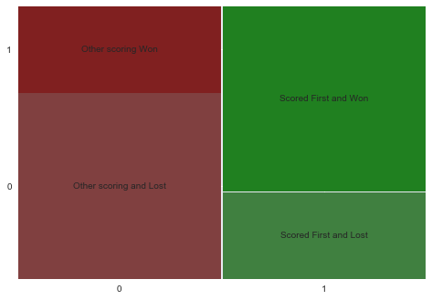
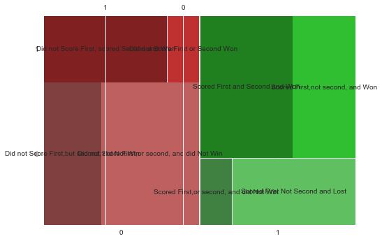
They are basically inverses of each other. The team that scored first and lost is the lower right hand corner. This matches our expectations, in that once you score it is hard to overcome, but not impossible. It would become even more impossible if they also scored second. But as you can see this produces a confusing plot with a number of contingencies.
labelizer=lambda k: {('1','0','0'): 'Scored First Not Second and Lost', ('1','1','1'): 'Scored First and Second and Won',
                     ('0','1','1'): 'Did not Score First, scored Second and Won',
           ('0','1','0'):"Did not Score First or Second Won",('0','0','1'):'Did not Score First,but second, did Not Win',
                     ('0','0','0'):'Did not Score First,or second, and did Not Win',
                    ('1','0','1'):'Scored First,or second, and did Not Win',
                    ('1','1','0'):'Scored First,not second, and Won',}[k]
mosaic(df, ['scoredfirst', 'won','scoredsecond'],labelizer=labelizer)
(<matplotlib.figure.Figure at 0x172eaf98>,
 OrderedDict([(('0', '0', '1'), (0.0, 0.0, 0.1832533523527387, 0.6799929876563392)), (('0', '0', '0'), (0.18435648414389383, 0.0, 0.31315595366705157, 0.6799929876563392)), (('0', '1', '1'), (0.0, 0.6833152467925517, 0.39525611070246164, 0.3166847532074481)), (('0', '1', '0'), (0.39635924249361676, 0.6833152467925517, 0.10115319531732865, 0.3166847532074481)), (('1', '0', '1'), (0.5024875621890548, 0.0, 0.10115319531732864, 0.3166847532074481)), (('1', '0', '0'), (0.6047438892975385, 0.0, 0.39525611070246164, 0.3166847532074481)), (('1', '1', '1'), (0.5024875621890548, 0.32000701234366075, 0.2951368258328812, 0.6799929876563392)), (('1', '1', '0'), (0.7987275198130911, 0.32000701234366075, 0.20127248018690908, 0.6799929876563392))]))
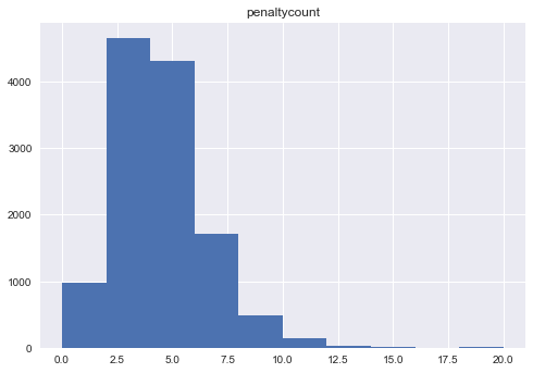
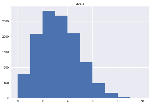
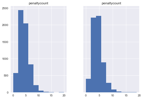
There are very few numeric variables in the dataset, but it is worth reviewing those as well. Below are the histograms for the number of goals and the number of penalties teams receive. Overall, teams tend to receive between 2 and 7 penalties a game. It is much more rare to have teams that have more than 10 goals in a game. The number of goals is also around 2 to 5. Somewhat supporting that the NHL is a low scoring game.
df.hist('penaltycount')
df.hist('goals')
array([[<matplotlib.axes._subplots.AxesSubplot object at 0x00000000176B8C88>]],
      dtype=object)
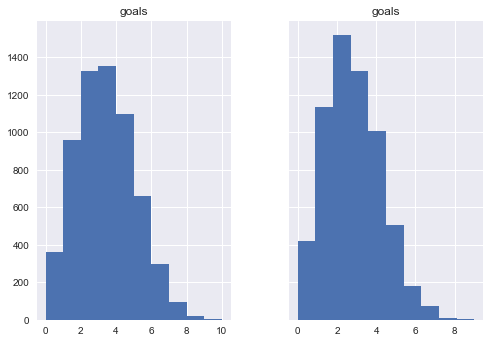
We can also break this up by whether it was a home game.
f, (ax1, ax2) = plt.subplots(1, 2, sharey=True)
print "Mean Home Penalty %s"%df[df['home']==1]['goals'].mean()
print "Mean Not Home Penalty %s"%df[df['home']==0]['goals'].mean()
df[df['home']==1].hist('goals',ax=ax1)
df[df['home']==0].hist('goals',ax=ax2)
Mean Home Penalty 2.92052444157
Mean Not Home Penalty 2.65053415345


array([<matplotlib.axes._subplots.AxesSubplot object at 0x000000001980FE80>],
      dtype=object)
f, (ax1, ax2) = plt.subplots(1, 2, sharey=True)
print "Mean Home Penalty %s"%df[df['home']==1]['penaltycount'].mean()
print "Mean Not Home Penalty %s"%df[df['home']==0]['penaltycount'].mean()
df[df['home']==1].hist('penaltycount',ax=ax1)
df[df['home']==0].hist('penaltycount',ax=ax2)
Mean Home Penalty 3.83505988993
Mean Not Home Penalty 4.13386209129


array([<matplotlib.axes._subplots.AxesSubplot object at 0x0000000017D846D8>],
      dtype=object)
print "Mean Home Wins %s"%df[df['home']==1]['won'].mean()
print "Mean Not Home Wins %s"%df[df['home']==0]['won'].mean()
print "Overtime %s"%df[df['won']==1]['overtime'].mean()
print "Mean Period for Wins %s"%df[df['won']==1]['period'].mean()
print "Mean Period for Not Wins %s"%df[df['won']==0]['period'].mean()

print "Mean Period for Wins %s"%df[(df['won']==1)&(df['scoredfirst']==1)]['period'].mean()
print "Mean Period for Not Wins %s"%df[(df['won']==0)&(df['scoredfirst']==1)]['period'].mean()
Mean Home Wins 0.546617028164
Mean Not Home Wins 0.453382971836
Overtime 0.131757850437
Mean Period for Wins 1.24878601489
Mean Period for Not Wins 1.24878601489
Mean Period for Wins 1.27141162515
Mean Period for Not Wins 1.20020376974
There are a total 6166 games in the dataset. On average the winning team wins by 2 goals, and on average away teams score 2 goals and home teams score 2 goals. Both these might be rounded up to 3 goals. I’m not sure that the difference in the number of goals is statistically significant, though. Home teams won about 55% of the games in the dataset. That is pretty close to a 50/50 chance of winning at home. There are some arguments in sports that home teams always perform better than away teams, so-called home field (ice) advantage. Although, at the same time crowds appear to have little affect on the players, and the suggestion is the crowds influence the refs to favor the home team. Not purposeful, as in the refs are cheating, but through social preassure (having 15,000 people yelling “ref you suck” for example). At least, that is the case argued in Soccernomics. It isn’t clear that there isn’t much of a home ice advantage in terms of win percentage.
Also, a small proportion of winning games go into overtime, 13%. So most regular season games end with a winner after three periods.
Important for the task at hand, is more than about 67% of the game winners also scored first, and about 40% of those game winners also scored the second goal scored.
Again, intuitively this makes sense. Once they score, it is harder for the opposing team to overcome this. But it appears only a little bit harder. If we round down then that would be 6 out of 10 winning teams likely scored first.
That first goal on average comes in the first period.
Who Scores First?
A second question is, is there any distinction between who scores the first goal. This could be of real value to a team. Are there skaters that are really good at breaking the ice? My initial guess would be that the top scorers in the league will top this list. There are different ways to brek this up, but I’m going to include the goal scorer and those that assist. If you’ve watched ice hockey before then you know the one credited with the goal may have tipped in or redirected a shot. So the assists are just as important as those that get the main credit.
To get the scorer, I use a regular expression search to parse out the information. This was simpler than trying to spilt multiple times. Luckily the description followed a similar pattern with similar literals.
ls = pickle.load(open('firstGoalDesc2015.p','rb'))
scores = []
scores_teams = []
assists = []
assists_teams = []
for s in ls:
    team = s[2][:3]

    sections = s[2].split(",")
    line = sections[0]
    line = line.replace("'","")
    mo = re.search(r'#\d{1,2}\s?([\w\s]+)', line)
    scores.append(team + " " + mo.group(1))
    scores_teams.append(team)
    #print line
    #print mo.group()
    #print mo.group(1)
    for line in sections:
        if "assists" in line.lower():
            assistLines = line.split(";")
            for al in assistLines:
                al = al.replace("'","")
                mo = re.search(r'#\d{1,2}\s([\w\s]+)', al)
                assists.append(team + " " + mo.group(1))
                assists_teams.append(team)
df_s = pd.DataFrame({'scores':scores+assists,"teams":scores_teams+assists_teams})
print df_s.head()
print df_s['teams'].unique()
df_scnt = pd.DataFrame(pd.value_counts(df_s['scores'].values.ravel()) .reset_index())
df_scnt.columns = ['scorer', 'count']
print df_scnt.hist('count')
print df_scnt.head()
print df_scnt['count'].mean()
1-poisson.cdf(8, df_scnt['count'].mean())
           scores teams
0  MTL PACIORETTY   MTL
1       BOS SMITH   BOS
2     VAN BURROWS   VAN
3     S.J WINGELS   S.J
4      CBJ SKILLE   CBJ
['MTL' 'BOS' 'VAN' 'S.J' 'CBJ' 'N.J' 'PIT' 'WSH' 'FLA' 'NYR' 'OTT' 'CHI'
 'MIN' 'CGY' 'WPG' 'NYI' 'ANA' 'T.B' 'PHI' 'STL' 'DAL' 'L.A' 'EDM' 'TOR'
 'COL' 'BUF' 'NSH' 'CAR' 'DET' 'ARI']
[[<matplotlib.axes._subplots.AxesSubplot object at 0x00000000199D2438>]]
          scorer  count
0       DAL BENN     20
1  PIT HORNQVIST     19
2     OTT TURRIS     18
3    OTT HOFFMAN     17
4    NYI TAVARES     17
4.55555555556


0.042887035129762885
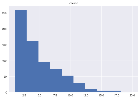
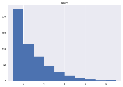
The histogram shows this follows more of a poisson distribution, so I can use that to see what might be the extreme values, e.g. scorers\assists who tend to have a high number of first score goals. In 2014, the cut off is about 8 goals and or assists.
df_scnt[df_scnt['count']>=8].head(10)
| scorer | count | |
|---|---|---|
| 0 | DAL BENN | 20 |
| 1 | PIT HORNQVIST | 19 |
| 2 | OTT TURRIS | 18 |
| 3 | OTT HOFFMAN | 17 |
| 4 | NYI TAVARES | 17 |
| 5 | STL TARASENKO | 17 |
| 6 | CAR STAAL | 17 |
| 7 | VAN SEDIN | 16 |
| 8 | DAL SEGUIN | 16 |
| 9 | PIT CROSBY | 15 |
If you follow ice hockey, then the names you see in the top ten should not be a big surprise. They are some of the leagues top players, and more so in 2014-2015 (Been, Tarsenko, Tavares, Crosby). Most of the teams in the top ten also made it to the plays. As the table below (Source: https://en.wikipedia.org/wiki/2014%E2%80%9315_NHL_season) shows, a number of the names appear again.
| Player | Team | GP | G | A | Pts | +/– | PIM |
|---|---|---|---|---|---|---|---|
| Jamie Benn | Dallas Stars | 82 | 35 | 52 | 87 | +1 | 64 |
| John Tavares | New York Islanders | 82 | 38 | 48 | 86 | +5 | 46 |
| Sidney Crosby | Pittsburgh Penguins | 77 | 28 | 56 | 84 | +5 | 47 |
| Alexander Ovechkin | Washington Capitals | 81 | 53 | 28 | 81 | +10 | 58 |
| Jakub Voracek | Philadelphia Flyers | 82 | 22 | 59 | 81 | +1 | 78 |
| Nicklas Backstrom | Washington Capitals | 82 | 18 | 60 | 78 | +5 | 40 |
| Tyler Seguin | Dallas Stars | 71 | 37 | 40 | 77 | −1 | 20 |
| Jiri Hudler | Calgary Flames | 78 | 31 | 45 | 76 | +17 | 14 |
| Daniel Sedin | Vancouver Canucks | 82 | 20 | 56 | 76 | +5 | 18 |
| Vladimir Tarasenko | St. Louis Blues | 77 | 37 | 36 | 73 | +27 | 31 |
We might ignore VAN SEDIN because there are actually two Sedins (Twins) that played for Vancouver. It is like this number is inflated a little because of this. Still according to the wikipedia page Daniel Sedin made a number of goals and assists.
Turris and Hoffman both played for Ottawa and both had over 20 goals that season, but Ottawa did not make the playoffs. Niether did Carolina, but the other teams do.
Interestingly, high goal scorers like Ovechkin don’t crack the top ten in this season at least. It’s likely his goals come later in the game.
ls = pickle.load(open('firstGoalDesc2018.p','rb'))
scores = []
scores_teams = []
assists = []
assists_teams = []
for s in ls:
    team = s[2][:3]

    sections = s[2].split(",")
    line = sections[0]
    line = line.replace("'","")
    mo = re.search(r'#\d{1,2}\s?([\w\s]+)', line)
    scores.append(team + " " + mo.group(1))
    scores_teams.append(team)
    #print line
    #print mo.group()
    #print mo.group(1)
    for line in sections:
        if "assists" in line.lower():
            assistLines = line.split(";")
            for al in assistLines:
                al = al.replace("'","")
                mo = re.search(r'#\d{1,2}\s([\w\s]+)', al)
                assists.append(team + " " + mo.group(1))
                assists_teams.append(team)
df_s = pd.DataFrame({'scores':scores+assists,"teams":scores_teams+assists_teams})
print df_s.head()
print df_s['teams'].unique()
df_scnt = pd.DataFrame(pd.value_counts(df_s['scores'].values.ravel()) .reset_index())
df_scnt.columns = ['scorer', 'count']
print df_scnt.hist('count')
print df_scnt.head()
print df_scnt['count'].mean()
1-poisson.cdf(8, df_scnt['count'].mean())
df_scnt[df_scnt['count']>=8].head(10)
         scores teams
0     TOR KADRI   TOR
1   PIT SCHULTZ   PIT
2   EDM MCDAVID   EDM
3    PHI GIROUX   PHI
4  BOS PASTRNAK   BOS
['TOR' 'PIT' 'EDM' 'PHI' 'BOS' 'BUF' 'COL' 'OTT' 'DET' 'CHI' 'ARI' 'L.A'
 'CBJ' 'T.B' 'DAL' 'N.J' 'NYI' 'WSH' 'MIN' 'STL' 'WPG' 'NYR' 'CGY' 'MTL'
 'NSH' 'VGK' 'ANA' 'VAN' 'S.J' 'CAR' 'FLA']
[[<matplotlib.axes._subplots.AxesSubplot object at 0x000000001A2CED30>]]
         scorer  count
0    PHI GIROUX     21
1  T.B KUCHEROV     17
2   EDM MCDAVID     17
3     WPG LAINE     16
4   WPG WHEELER     16
4.51202263083
| scorer | count | |
|---|---|---|
| 0 | PHI GIROUX | 21 |
| 1 | T.B KUCHEROV | 17 |
| 2 | EDM MCDAVID | 17 |
| 3 | WPG LAINE | 16 |
| 4 | WPG WHEELER | 16 |
| 5 | NSH SUBBAN | 16 |
| 6 | COL RANTANEN | 16 |
| 7 | CBJ PANARIN | 15 |
| 8 | ARI KELLER | 15 |
| 9 | CHI KANE | 15 |
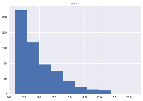
Different names come up each year. For 2017-2018 (missing Ovechkin again). Actually, neither team that made the final had a player that was really good at scoring first. That makes me suspect that it is less important during the playoffs, than it is during the regular season.
The list changes when the assists are taken out. But I think it is less valuable information. You want to know players that play an active role in getting that first goal.
df_s = pd.DataFrame({'scores':scores,"teams":scores_teams})
print df_s.head()
print df_s['teams'].unique()
df_scnt = pd.DataFrame(pd.value_counts(df_s['scores'].values.ravel()) .reset_index())
df_scnt.columns = ['scorer', 'count']
print df_scnt.hist('count')
print df_scnt.head()
print df_scnt['count'].mean()
df_scnt[df_scnt['count']>=8].head(10)
         scores teams
0     TOR KADRI   TOR
1   PIT SCHULTZ   PIT
2   EDM MCDAVID   EDM
3    PHI GIROUX   PHI
4  BOS PASTRNAK   BOS
['TOR' 'PIT' 'EDM' 'PHI' 'BOS' 'BUF' 'COL' 'OTT' 'DET' 'CHI' 'ARI' 'L.A'
 'CBJ' 'T.B' 'DAL' 'N.J' 'NYI' 'WSH' 'MIN' 'STL' 'WPG' 'NYR' 'CGY' 'MTL'
 'NSH' 'VGK' 'ANA' 'VAN' 'S.J' 'CAR' 'FLA']
[[<matplotlib.axes._subplots.AxesSubplot object at 0x000000001B2FBF98>]]
          scorer  count
0      WPG LAINE     11
1  MTL GALLAGHER     10
2      NSH SMITH     10
3      NYR HAYES      9
4  STL TARASENKO      9
2.40227703985
| scorer | count | |
|---|---|---|
| 0 | WPG LAINE | 11 |
| 1 | MTL GALLAGHER | 10 |
| 2 | NSH SMITH | 10 |
| 3 | NYR HAYES | 9 |
| 4 | STL TARASENKO | 9 |
| 5 | DAL SEGUIN | 8 |
| 6 | VGK TUCH | 8 |
| 7 | EDM MCDAVID | 8 |
| 8 | PHI GIROUX | 8 |
| 9 | MIN ZUCKER | 8 |
